from vectorbtpro import *

from datetime import datetime
from dateutil.relativedelta import relativedelta

from pypfopt.objective_functions import transaction_cost
from pypfopt import expected_returns, EfficientSemivariance
from pypfopt.risk_models import CovarianceShrinkage
from pypfopt.efficient_frontier import EfficientFrontier

vbt.settings.set_theme("dark")

Portfolio Optimization

Acknowledgements:

We will be using vector-bt, a (semi-)professional vectorized backtesting library written in Python, written by Oleg Polakow.

Note: For detailed documentation see documentation

Intro Portfolio Theory

Financial markets are highly nondeterministic. We want to find the portfolio that offers us high returns at low risk under the following market assumptions.

1. Rational decision-makers: Investors want to maximise return while reducing the risks associated with their investment
2. No arbitrage : cannot make a costless, riskless profit
3. Risky securities : $\{S_1,\ldots,S_n\}:\, n\geq 2$ be risky securities whose future returns are uncertain. There is no risk-free asset $S_0$ in our portfolio
4. Equilibrium : supply equals demand for securities
5. Liquidity : any # of units of a security can be bought and sold quickly
6. Access to information : rapid availability of accurate information
7. Price is efficient : Price of security adjusts immediately to new information, and current price reflects past information and expected further behaviour
8. No transaction costs and taxes : transaction costs are assumed to be negligible compared to value of trades (we may relax this assumption and assume cost $K$ per transaction) and are ignored. No taxes (capital-gains etc.) on transactions.

We want to select a portfolio $\mathbf{x}=(x_1,\ldots,x_n)\in\mathbb{R}^n$ where $x_i$ is the amount (fraction of budget) invested in security $S^i$. We work in discrete-time, so we only consider now ($t=0$) and a moment in time in the future ($t=1$)

The return of asset $i$ is a random variable $r_i:\Omega \rightarrow [0,\infty)$ where $\Omega$ is the sample space (set of scenarios for the future). If $S_t^i:\Omega\rightarrow\mathbb{R}_+$ is the random variable denoting the future value of asset $i$ at time $t$. Then under scenario $\omega\in\Omega$, we have that $r_i(\omega)=S^i_1(\omega)/S_0^i$. So for instance, a $5\%$ return on asset $i$ corresponds to $r_i=1.05$ and $-2%$ return corresponds to $r_i=0.98$

$\newcommand{\x}{\mathbf{x}}$ Let $r = (r_1,\ldots, r_n)$ denote the random vector of returns with mean $\mu=\mathbf{E}[r]\in\mathbb{R}^n$ and covariance matrix $\Sigma\in\mathbb{R}^{n\times n}$. Let the set of admissible portfolios be denoted by $X=\{\x\in\mathbb{R}^n:\sum_{i=0}^n x_i=1,\, \x\geq 0\}\subset\mathbb{R}^n$. In other words, we do not allow short-selling (for now), and must always be fully-allocated.

Then the return of portfolio $\mathcal{R}:X\rightarrow \mathbb{R}$ is given by $\mathcal{R}(\x)=r^T\x \implies \mathbf{E}[\mathcal{R}] = \mu^T\x$.

The risk of portfolio $\x\in X$ is denoted $\text{Risk}(\x)\equiv\text{Risk}(\mathcal{R}(\x))$ where $\text{Risk}:X\rightarrow\mathbb{R}$ is the risk measure.

$\newcommand{\x}{\mathbf{x}}$ $\newcommand{\y}{\mathbf{y}}$

$$ r_0 + \Bigl(\frac{\mathbf{E}[R(\x)]-r_0}{\sigma(\x)}\Bigr)\sigma(\y)\quad\text{where}\quad \y=(1-\alpha, \alpha\x) \tag{1} $$

$$ \text{SR}(\x) := \frac{\mathbf{E}[R(\x)]-r_0}{\sigma(\x)} \tag{2} $$

$$ \text{STR}(\x) := \frac{\mu^T\x-R}{\sqrt{\mathbf{E}(\min\{0,(r-\mu)^T\x\})^2}} \tag{3} $$

We seek the maximum slope of the the Capital Allocation Line (CAL) (1) which is the Sharpe Ratio (2). The Sortino ratio (3) penalizes only downside std. deviation (i.e. when $r^T\x < \mu^T\x$).

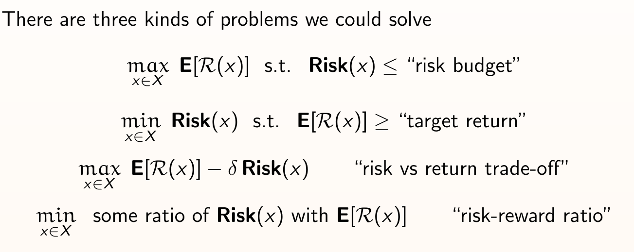
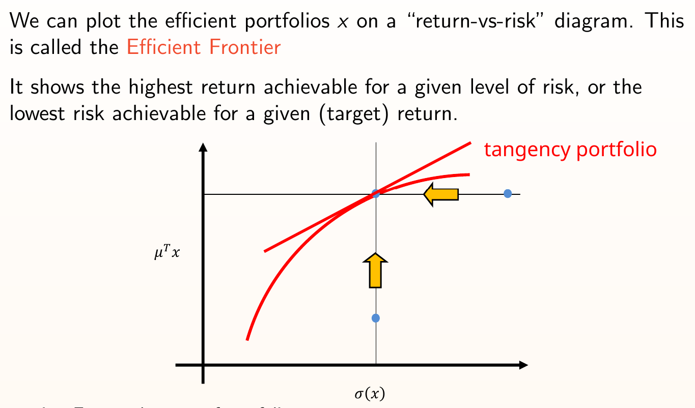
A portfolio is efficient if it has the maximum expected return among all admissible portfolios of the same (or smaller) risk: $\max \{\mu^T\x : \text{Risk}(\x)\leq \sigma^2,\, \x\in X\}$ or if it has the minimum variance among all admissible portfolios of the same (or greater) expected return: $\min\{ \text{Risk}(\x) : \mu^T\x\geq R,\, x\in X\}$. The efficient frontier is the set of all efficient portfolios.

Setup

END_DATE = datetime.today().strftime("%Y-%m-%d")
START_DATE = (datetime.today() - relativedelta(years=3)).strftime("%Y-%m-%d")

data = vbt.YFData.pull(
    ["BTC-USD", "ETH-USD", "XMR-USD", "LINK-USD"], 
    start=f"{START_DATE} UTC", 
    end=f"{END_DATE} UTC",
    timeframe="1d"
)

#data.to_hdf("data/YFData.h5") # save data to disk 
#data = vbt.HDFData.pull("data/BinanceData.h5") # retrieve data from disk

The object returned inherits from the vectorbtpro.data base class, which is very extensible, but for modeling purposes we only really care about OHLC data.

df = data.get("close")

def calc_returns(x : pd.Series) -> pd.Series:
    ret = (x.diff() / x.shift(1)).dropna()
    return ret

Risk-Return Tradeoff

$\newcommand{\x}{\mathbf{x}}$ $\newcommand{\R}{\mathbb{R}}$ $$ \max\; \{\mu^T\x -\delta\cdot\text{Risk}(x)\, |\, \x\in X \}\quad \text{where}\quad X=\{\x\in[-1,1]^n\, |\, \x^T\mathbf{1}=1 \} $$

def obj_func(x, mu, cov_matrix, delta):
    var = x.T @ (cov_matrix * np.eye(cov_matrix.shape[0])) @ x
    return -((mu.T @ x) - delta * var)

def optimize_func(price, index_slice):
    price_filt = price.iloc[index_slice]
    mu = expected_returns.mean_historical_return(price_filt)
    S = CovarianceShrinkage(price_filt).ledoit_wolf()
    ef = EfficientFrontier(mu, S, weight_bounds=(-1, 1))
    ef.convex_objective(obj_func, mu=mu.values, cov_matrix=S.values, delta=0.1)
    weights = ef.clean_weights()
    return weights

pfo = vbt.PortfolioOptimizer.from_optimize_func(
    data.symbol_wrapper,
    optimize_func,
    data.get("Close"),
    vbt.Rep("index_slice"),
    every="M"
)
pf = pfo.simulate(data, freq="1d")

print(f"SR: {pf.sharpe_ratio:.3f}, Sortino: {pf.sortino_ratio: .3f}\nMDD: {pf.max_drawdown*100: .2f}%, AR: {pf.annualized_return*100: .2f}%")

SR: 1.489, Sortino:  2.387
MDD: -35.12%, AR:  88.19%

Multiple Optimization

$\newcommand{\x}{\mathbf{x}}$ $$ \max\limits_{\x}\; \text{SR}(\x):=\frac{\mu^T \x - r_0}{\sqrt{\x^T\Sigma \x}}\quad \text{s.t.}\quad \x\in X:=\{\x\in[0,1]^n\, |\, \x^T\mathbf{1}=1 \} $$ $$ \min\limits_{\x}\; \x^T\Sigma\x\quad \text{s.t.}\quad \x\in X $$ $$ \min\limits_{\x}\; \frac{1}{2}\x^T Q\x + b^T\x + c\quad \text{s.t.}\quad \x\in X $$

pfo1 = vbt.PortfolioOptimizer.from_pypfopt(
    prices=data.get("Close"),
    every="1M",
    weight_bounds=(0, 1),
    target=vbt.Param([
        "max_sharpe",
        "min_volatility",
        "max_quadratic_utility",
    ]),
)

# get portfolio performance for each target
pf1 = pfo1.simulate(data, freq="1d")
print(f"{pf1.sharpe_ratio}\n\n{pf1.max_drawdown}\n\n{pf1.annualized_return}")

target
max_sharpe               1.251148
min_volatility           0.848033
max_quadratic_utility    1.001655
Name: sharpe_ratio, dtype: float64

target
max_sharpe              -0.560882
min_volatility          -0.426625
max_quadratic_utility   -0.577339
Name: max_drawdown, dtype: float64

target
max_sharpe               0.865026
min_volatility           0.331285
max_quadratic_utility    0.585985
Name: annualized_return, dtype: float64

# compare performance against buy-and-hold strategy for S&P 500 
benchmark_data = vbt.YFData.pull(
    "SPY",
    start=f"{START_DATE} UTC", 
    end=f"{END_DATE} UTC",
    timeframe="1d",
    tz='UTC'
)
bm_close = benchmark_data.get('Close')
bm_close.index = bm_close.index.normalize() # remove market close timestamp

fig = vbt.make_subplots(rows=1, cols=2)
fig.update_layout(width=1000,height=400)
pf1.plot_cumulative_returns(column=1, bm_returns=calc_returns(bm_close), add_trace_kwargs=dict(row=1, col=1), fig=fig)
pfo1.plot(column=1, add_trace_kwargs=dict(row=1, col=2), fig=fig)
fig.show()

So the Sharpe ratio $S_a=1.24$ is not ideal if we're chasing alpha (i.e. profitable strategy whether the market is bearish/bullish), but if we're just looking to increase our beta (increasing exposure to the market swings to capture the most price action) then this is starting to look better. Note that we also outperform a buy-and-hold strategy on the S&P 500.

initial_weights = np.array([1 / len(data.symbols)] * len(data.symbols))
pfo2 = vbt.PortfolioOptimizer.from_pypfopt(
    prices=data.get("Close"),
    every="1M",
    weight_bounds=(-1, 1),
    objectives=["transaction_cost"],
    w_prev=initial_weights, 
    k=0.001,
    target=vbt.Param([
        "max_sharpe", 
        "min_volatility", 
        "max_quadratic_utility"
    ])
)

pf2 = pfo2.simulate(data, freq="1d")
print(f"{pf2.sharpe_ratio}\n\n{pf2.sortino_ratio}\n\n{pf2.max_drawdown}\n\n{pf2.annualized_return}")

target
max_sharpe               0.627570
min_volatility           0.728677
max_quadratic_utility    1.393467
Name: sharpe_ratio, dtype: float64

target
max_sharpe               0.969260
min_volatility           1.033604
max_quadratic_utility    2.201139
Name: sortino_ratio, dtype: float64

target
max_sharpe              -0.409129
min_volatility          -0.342790
max_quadratic_utility   -0.407796
Name: max_drawdown, dtype: float64

target
max_sharpe               0.203743
min_volatility           0.242462
max_quadratic_utility    0.764997
Name: annualized_return, dtype: float64

If we consider a per-trade transction cost of $0.1\%$ of the amount traded, the story changes; we now are actually less profitable with an atrocious decrease of $> 60\%$ in annualized returns (for a max_sharpe optimization objective).

However, in optimizing for minimum volatility, including transaction fees only shifts the annualized returns down by about $10\%$.

Efficient Semivariance

$$ \min\limits_{x}\; \mathbf{E}[((\mu-x)^+)^2]\quad\text{s.t.}\quad\x\in X $$

pfo3 = vbt.PortfolioOptimizer.from_pypfopt(
    prices=data.get("Close"),
    every="1M",
    weight_bounds=(0, 1),
    objectives=["transaction_cost"],
    w_prev=initial_weights, 
    k=0.001,
    target="efficient_return",
    target_return=0.01,
    optimizer="efficient_semivariance",  
    lookback_period="2M",
)
pf3 = pfo3.simulate(data, freq="1d")

print(f"SR: {pf.sharpe_ratio:.3f}, Sortino: {pf.sortino_ratio: .3f}\nMDD: {pf.max_drawdown*100: .2f}%, AR: {pf.annualized_return*100: .2f}%")

SR: 1.489, Sortino:  2.387
MDD: -35.12%, AR:  88.19%

fig = vbt.make_subplots(rows=1, cols=2)
fig.update_layout(width=1000,height=400)
pf3.plot_cumulative_returns(bm_returns=calc_returns(bm_close), add_trace_kwargs=dict(row=1, col=1), fig=fig)
pfo3.plot(add_trace_kwargs=dict(row=1, col=2), fig=fig)
fig.show()

In optimizing for efficient semivariance (i.e. finding the efficient portfolio with the minimum downside deviation), we achieve an adequate sharpe ratio of $SR(\mathbf{x})=1.48$, while outperforming a buy-and-hold strategy on the S&P 500.

Conclusion

Optimizing portfolios for certain target metrics periodically and rebalancing can lead to promising results for beta-seeking strategies. However this all depends on the optimization constraints, the target parameter, and of course the assets considered.

For those of you interested, there is web-app service called Portfolio Visualizer where you can optimize portfolios subject to different constraints.

Disclaimer:

Please do not distribute this notebook.

The analysis in this material is provided for information only and should not be construed as advice to buy any cryptocurrency